Doubling of coastal flooding frequency within decades due to sea-level rise

Global climate change drives sea-level rise, increasing the frequency of coastal flooding. In most coastal regions, the amount of sea-level rise occurring over years to decades is significantly smaller than normal ocean-level fluctuations caused by tides, waves, and storm surge. However, even gradual sea-level rise can rapidly increase the frequency and severity of coastal flooding. So far, global-scale estimates of increased coastal flooding due to sea-level rise have not considered elevated water levels due to waves, and thus underestimate the potential impact. Here we use extreme value theory to combine sea-level projections with wave, tide, and storm surge models to estimate increases in coastal flooding on a continuous global scale. We find that regions with limited water-level variability, i.e., short-tailed flood-level distributions, located mainly in the Tropics, will experience the largest increases in flooding frequency. The 10 to 20 cm of sea-level rise expected no later than 2050 will more than double the frequency of extreme water-level events in the Tropics, impairing the developing economies of equatorial coastal cities and the habitability of low-lying Pacific island nations.

Global sea level is currently rising at ~3–4 mm/yr^{1, 2} and is expected to accelerate due to ocean warming and land-based ice melt^{3, 4}. Sea-level rise (SLR) projections range from 0.3 to 2.0 m by 2100, depending on methodology and emission scenarios^{5, 6}, and recent work suggests that accepted methodologies significantly underestimate the contribution of Antarctica⁷.
Coastal regions experience elevated water levels on an episodic basis due to wave setup and runup⁸, tides⁹, storm surge driven by wind stress and atmospheric pressure, contributions from seasonal and climatic cycles, e.g., El Niño/Southern Oscillation^{10, 11} and Pacific Decadal Oscillation¹², and oceanic eddies¹³ (Fig. 1).

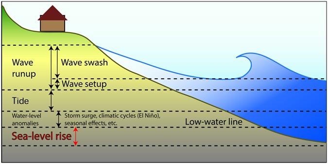
Coastal flooding often occurs during extreme water-level events that result from simultaneous, combined contributions, such as large waves, storm surge, high tides, and mean sea-level anomalies^{11, 14}.
SLR leads to (1) passive high-tide inundation of low-lying coastal areas¹⁵, (2) increased frequency, severity, and duration of coastal flooding¹⁶, (3) increased beach erosion¹⁷, (4) groundwater inundation^{18, 19}, (5) changes to wave dynamics²⁰, and (6) displacement of communities²¹. Predicting regions vulnerable to passive inundation is relatively simple with the aid of high-resolution digital elevation models²². However, predicting the effect of SLR on episodic flooding events is difficult due to the unpredictable nature of coastal storms, nonlinear interactions of physical processes (e.g., tidal currents and waves), and variations in coastal geomorphology (e.g., sediments, bathymetry, topography, and bed friction). Local-scale assessments of coastal hazard vulnerability typically rely on detailed, computationally-onerous numerical modeling efforts²³ in order to simulate wave-related nearshore water levels, interactions with local topography, and the resulting flooding. Global-scale coastal hazard vulnerability assessments, on the other hand, rely on extreme value theory applied to water-level observations.

Extreme-value theory

Extreme-value theory^{24, 25} is a statistical method for quantifying the probability or return period of large events. The generalized extreme value (GEV) distribution, sometimes called the Fisher-Tippet distribution, is a powerful and general statistical model for extremes²⁶ (Coles 2001). The GEV distribution models the probabilities of the maxima of a random variable^{24, 27, 28} using three parameters μ, σ, and k, the location (mean), scale (width), and shape (family type), respectively²⁶.
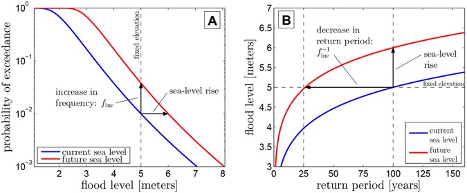
Oceanographic and coastal engineering studies often rely on GEV theory to describe the frequency of extreme waves²⁹, water-level events³⁰, flooding impacts³¹, and to understand the effects of SLR³². As sea level increases, the probability increases that a fixed elevation will experience flooding (Fig. 2). Equivalently, the return period or recurrence interval of flooding at a fixed elevation decreases^{33, 34}. In the example shown in Fig. 2B, 1 m of SLR causes the 5 m flood level (the former 100-year flood) to recur every 25 years.

SLR can affect flood magnitude and frequency directly (Fig. 2) or indirectly via hydrodynamic feedbacks: SLR alters water depths, changing the generation, propagation, and interaction of waves, tides, and storm surges. Thus, SLR and long-term changes in wave climate, e.g., changes in magnitude, frequency, and tracks of storms^35,36,37 and storm surge, can alter the parameters of extreme water-level distributions and the evolution of coastal hazards over time. In the proposed work, we assume parameter stationarity based on projections of minor changes (5–10%^35,36,37) in mean annual wave conditions and storm surge over large regions of the ocean. In specific locations, such as the Pacific Northwest, trends in extreme wave climate may be significant³⁸ and lead to a greater flooding hazard than SLR over at least the next several decades³⁹, calling for nonstationary methods⁴⁰ in future research.
Investigations of increased flooding frequency due to SLR are often site-specific and rely only on water-level data from tide stations. For example, Hunter (2012) [ref. 41] and the Intergovernmental Panel on Climate Change (IPCC) 2013 report³ estimate the factor of increase in the frequency of flooding events due to 0.5 m of SLR at locations of 198 tide stations around the globe [Hunter⁴¹ Fig. 4 and IPCC³ Fig. 13.25]. Hunter⁴¹ and IPCC³ found that regions with low variability of extreme water levels will experience large increases in flooding frequency. This finding, introduced qualitatively by Hoozemans et al. [ref. 33], is critical to predict the global regions most vulnerable to SLR. However, global-scale coastal hazard assessments using this methodology encounter three challenges: (1) Water-level observation stations are sparsely located around the globe, especially in the Indian Ocean and South Atlantic; (2) wave-driven water-level contributions, i.e., setup and swash, are not included; and (3) the global variability of the GEV shape parameter has not been considered, although it can be as influential as the scale parameter in determining vulnerability. Here we meet the three challenges by using extreme-value theory to combine sea level, wave, tide, and storm-surge models to predict increases in extreme water-level frequency on a global scale.

Application

Flooding results from the complex interaction of extreme water levels, topography, and the built environment. Here we use the frequency of extreme water levels as a proxy for regional-scale increases in flooding frequency, while recognizing that the relationship between water level and flooding is location dependent because of coastal topography, coastal defense structures, and drainage systems.
We apply sea-level projections and global wave, tide, and storm surge models to predict the future return periods (associated with the former 50-yr extreme water level) due to SLR. As in Hunter⁴¹ and IPCC³, we begin by investigating increases in flooding frequency due to a globally-uniform amount of SLR, acknowledging that spatial variability in the regional rate of SLR (e.g., driven by ocean circulation patterns, glacial fingerprinting) and the local relative rate of SLR (e.g., due to tectonic activity, glacial isostasy, land subsidence) will affect flooding predictions for specific locations⁴². Later we take the inverse approach, estimating the amount of SLR that doubles the frequency of extreme water-level events.
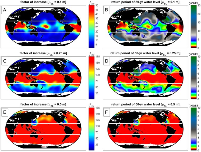
Using maximum likelihood estimates, we fit GEV probability distributions to the top three annual maximum water-level events from 1993–2013 obtained via synthesis of the Global Ocean Wave (GOW) reanalysis⁴³, Mog2D storm-surge model⁴⁴, and TPXO tide model⁴⁵ as discussed in Methods. Figure 3 shows the global variability of the mean (μ), scale (σ), and shape (k) parameters for extreme total water level in panels A, B, and C, respectively. The GEV parameters provide necessary inputs to the factors of increase, f _inc , and the future return period of the former 50-yr water level based on Eq. (3) (see Methods). Figure 4 shows the factor of increase for the SLR projections μ _SL  = +0.1, +0.25, +0.5 m on a global scale. Finally, the GEV parameters allow for global estimation of the amount of SLR that doubles the exceedance probability of the 50-yr water-level elevation [see Fig. 5 and Methods Eq. (4)]. Analyzing the amount of SLR leading to a doubling in flooding (Fig. 5) is equivalent to the factor-of-increase results shown in Fig. 4, but it provides a more intuitive picture of the effects of small amounts of SLR. Table 1 summarizes the global, tropical, and extra-tropical mean values of the quantities presented in Figs 3 and 5. Although the plotted distributions apply only to coasts, they are calculated ocean-wide in order to reveal the continuous global pattern of vulnerability of both continental coastal settings and non-contiguous island nations throughout the world’s oceans.